library(dplyr)

Attaching package: 'dplyr'

The following objects are masked from 'package:stats':

    filter, lag

The following objects are masked from 'package:base':

    intersect, setdiff, setequal, union

library(tidyverse)

── Attaching core tidyverse packages ──────────────────────── tidyverse 2.0.0 ──
✔ forcats   1.0.0     ✔ readr     2.1.5
✔ ggplot2   3.5.1     ✔ stringr   1.5.1
✔ lubridate 1.9.3     ✔ tibble    3.2.1
✔ purrr     1.0.2     ✔ tidyr     1.3.1

── Conflicts ────────────────────────────────────────── tidyverse_conflicts() ──
✖ dplyr::filter() masks stats::filter()
✖ dplyr::lag()    masks stats::lag()
ℹ Use the conflicted package (<http://conflicted.r-lib.org/>) to force all conflicts to become errors

library(stringr)
library(wordcloud2)
library(ggplot2)
df <- read_csv("data/movie.csv")

Rows: 1072255 Columns: 42
── Column specification ────────────────────────────────────────────────────────
Delimiter: ","
chr  (28): title, status, backdrop_path, homepage, imdb_id, original_languag...
dbl  (12): id, vote_average, vote_count, revenue, runtime, budget, popularit...
lgl   (1): adult
date  (1): release_date

ℹ Use `spec()` to retrieve the full column specification for this data.
ℹ Specify the column types or set `show_col_types = FALSE` to quiet this message.

df_clean <- read_csv("data/df_clean.csv")

New names:
Rows: 312801 Columns: 9
── Column specification
──────────────────────────────────────────────────────── Delimiter: "," chr
(4): title, status, genre, country dbl (5): ...1, year, revenue, budget, rate
ℹ Use `spec()` to retrieve the full column specification for this data. ℹ
Specify the column types or set `show_col_types = FALSE` to quiet this message.
• `` -> `...1`

Q1

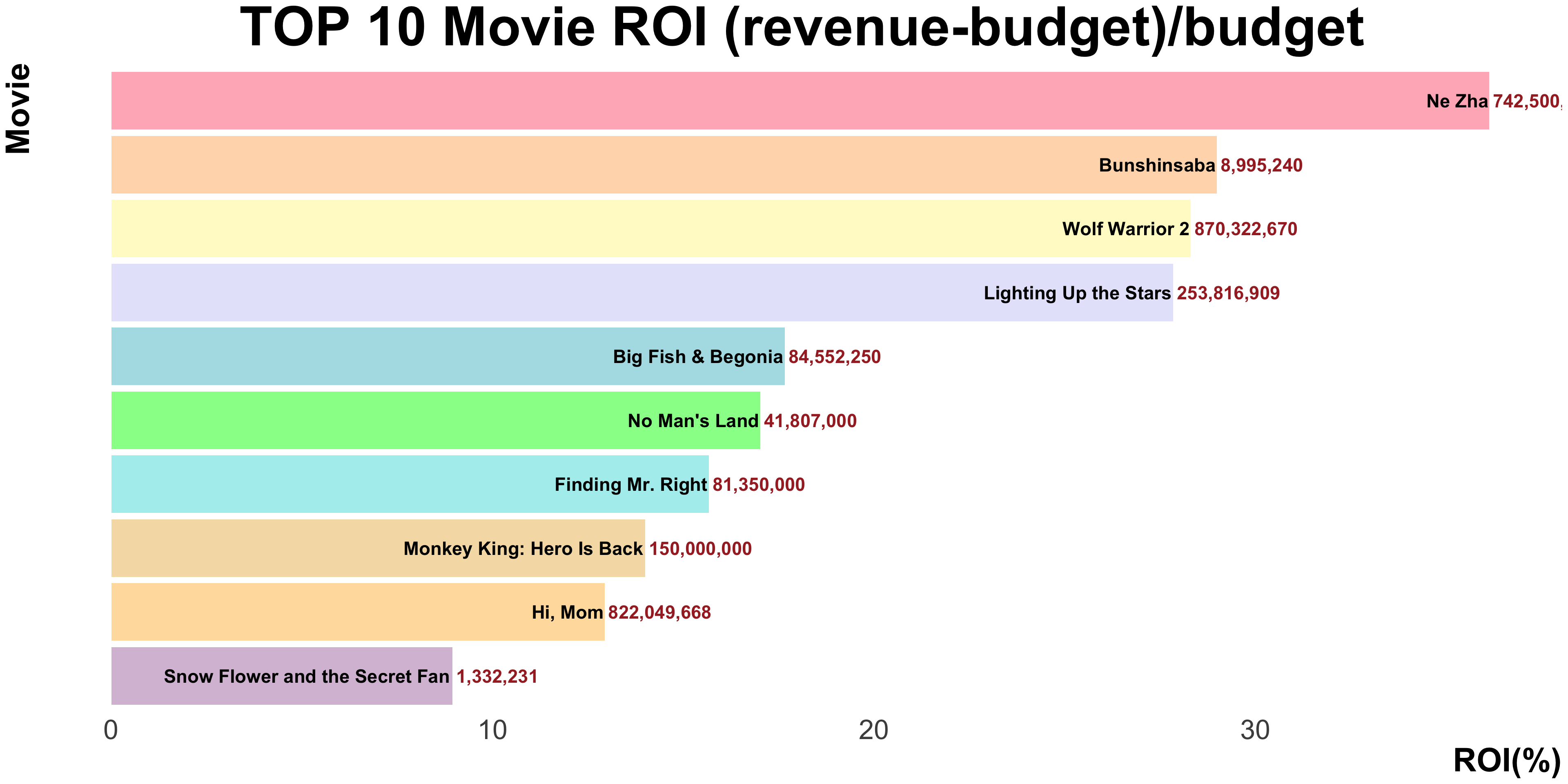
What are the top 10 most profitable movies in China over the past 20 years?

df1 <- df_clean |>
  filter(country == "China") |>
  #删掉revenue和budget=0的row
  filter(!(revenue == "0"))|>
  filter(!(budget == "0"))|>
  #创造一列ROI=((revenue-budget)/budget)
  mutate(ROI = (revenue - budget) / budget)|>
  #删除budget是的row(nchar:字符串长度/数字位数)
  filter(nchar(as.character(budget)) > 3) |>
  group_by(year) |>
  select(year, title, genre, ROI, revenue, budget)|>
  arrange(-ROI)|>
#However, since The revenue and budget of No.1 The Loony Park（马赛克大乱斗） and No.11 Sweet Journey（云下的日子） were obviously wrong, we removed these two films from the table.
  filter(!(title == "The Loony Park"))|>
  filter(!(title == "Sweet Journey"))|>
  filter(ROI>7.1892407)|>
  select(title, ROI, revenue)

Adding missing grouping variables: `year`

glimpse(df1)

Rows: 10
Columns: 4
Groups: year [9]
$ year    <dbl> 2019, 2012, 2017, 2022, 2016, 2013, 2013, 2015, 2021, 2011
$ title   <chr> "Ne Zha", "Bunshinsaba", "Wolf Warrior 2", "Lighting Up the St…
$ ROI     <dbl> 36.125000, 28.984133, 28.303794, 27.842831, 17.658147, 17.0202…
$ revenue <dbl> 742500000, 8995240, 870322670, 253816909, 84552250, 41807000, …

colors <- c(
  "#FFB6C1", "#FFDAB9", "#FFFACD", "#E6E6FA", "#B0E0E6",
  "#98FB98", "#AFEEEE", "#F5DEB3", "#FFDEAD", "#D8BFD8",
  "#FFC0CB", "#ADD8E6", "#87CEFA", "#FAFAD2", "#F0E68C",
  "#E0FFFF", "#D1EEEE", "#C1FFC1", "#FFF0F5", "#FFFAFA"
)

color1 <- c(
  "#FFB6C1", "#FFDAB9", "#FFFACD", "#E6E6FA", "#B0E0E6",
  "#98FB98", "#AFEEEE", "#F5DEB3", "#FFDEAD", "#D8BFD8"
)

ggplot(df1, aes(
  x = ROI, y = reorder(title, ROI), fill = reorder(title, -ROI) 
)) +
  geom_bar(stat = "identity", width = 0.9) +  
  geom_text(aes(label = title, x = ROI),     
            color = "black",                 
            size = 6,                      
            hjust = 1.008,                       
            fontface = "bold") +             

  geom_text(aes(label = scales::comma(revenue), x = ROI+0.1),
            color = "brown",                 
            size = 6,                       
            hjust = 0,                      
            fontface = "bold") +             
  scale_fill_manual(values = color1) +      
  labs(
    title = "TOP 10 Movie ROI (revenue-budget)/budget",
    x = "ROI(%)",
    y = "Movie"
  ) +
  theme_minimal() +
  theme(
    panel.grid = element_blank(),         
    axis.ticks.y = element_blank(),       
    axis.text.y = element_blank(),
    axis.text.x = element_text(size = 25),
    legend.position = "none" ,
    axis.title.x = element_text(        
      size = 30,                            
      face = "bold",
      hjust = 1
    ),
    axis.title.y = element_text(            
      size = 30,                            
      face = "bold",                        
      angle = 90,
      hjust = 1
    ),
    

    plot.title = element_text(        
      size = 50,  
      face = "bold",        
      hjust = 0.5              
    )
  )

ggsave(
  filename = "data/Q1.png",
  plot = last_plot(),             
  width = 20,                       
  height = 10,                    
  dpi = 300                         
)

Q2

How has the proportion of Chinese movie market changed in the past ten years?

df2 <- df_clean |>
  select(country, year, revenue) |>
  filter(year>2013)|>
  filter(!(year>2023))|>
  group_by(country, year) |>
  summarise(total_revenue = sum(revenue))

`summarise()` has grouped output by 'country'. You can override using the
`.groups` argument.

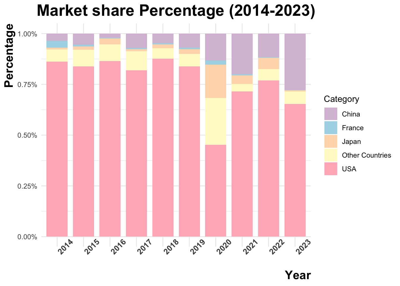
df2 <- df2 |>
  mutate(
    category = case_when(
      country == "China" ~ "China",
      country == "United States of America" ~ "USA",
      country == "France" ~ "France",
      country == "Japan" ~ "Japan",
      TRUE ~ "Other Countries"))

df2 <- df2 |>
  group_by(category,year) |>
  summarise(total_revenue = sum(total_revenue))

`summarise()` has grouped output by 'category'. You can override using the
`.groups` argument.

print(df2)

# A tibble: 50 × 3
# Groups:   category [5]
   category  year total_revenue
   <chr>    <dbl>         <dbl>
 1 China     2014     744883919
 2 China     2015    1185951291
 3 China     2016     441680092
 4 China     2017    1720894151
 5 China     2018    1173818739
 6 China     2019    1663018812
 7 China     2020     521570577
 8 China     2021    2472642884
 9 China     2022    2149167889
10 China     2023    3342450960
# ℹ 40 more rows

glimpse(df2)

Rows: 50
Columns: 3
Groups: category [5]
$ category      <chr> "China", "China", "China", "China", "China", "China", "C…
$ year          <dbl> 2014, 2015, 2016, 2017, 2018, 2019, 2020, 2021, 2022, 20…
$ total_revenue <dbl> 744883919, 1185951291, 441680092, 1720894151, 1173818739…

color2 <- c(
  "China" = "#D8BFD8",       
  "USA" = "#FFB6C1",        
  "France" = "#ADD8E6",
  "Japan" = "#FFDAB9",       
  "Other Countries" = "#FFFACD" 
  )

df2.2<- df2|>
  group_by(year) |>
  mutate(percentage = total_revenue / sum(total_revenue) * 100) |>
  ungroup()

ggplot(df2.2, aes(x = factor(year), y = percentage, fill = category)) +
  geom_bar(stat = "identity", position = "fill", width = 0.8) +  
  scale_y_continuous(labels = scales::percent_format(scale = 1)) + 
  scale_fill_manual(values = color2) +
  labs(
    title = "Market share Percentage (2014-2023)",
    x = "Year",
    y = "Percentage",
    fill = "Category"
  ) +
  theme_minimal() +
  theme(
    plot.title = element_text(hjust = 0.5, size = 20, face = "bold"),
    axis.text.x = element_text(angle = 45, size = 10, hjust = 0,  face = "bold"),
    axis.title.x = element_text(size = 15,face = "bold",hjust = 1),
    axis.title.y = element_text(            
      size = 15,                            
      face = "bold",                        
      angle = 90,
      hjust = 1
    )

  )

ggsave(
  filename = "data/Q2.png",
  plot = last_plot(),     
  width = 10, height = 6, dpi = 300     
)

Q3

What is the total number of films shown in each country? Where does China stand?

library(rnaturalearth)
library(rnaturalearthdata)

Attaching package: 'rnaturalearthdata'

The following object is masked from 'package:rnaturalearth':

    countries110

library(sf)

Linking to GEOS 3.11.0, GDAL 3.5.3, PROJ 9.1.0; sf_use_s2() is TRUE

df3 <- df_clean |>
  select(year, title, country) |>         
  group_by(country) |>
  summarise(number = n())  |>
  arrange(-number)
print(df3)

# A tibble: 232 × 2
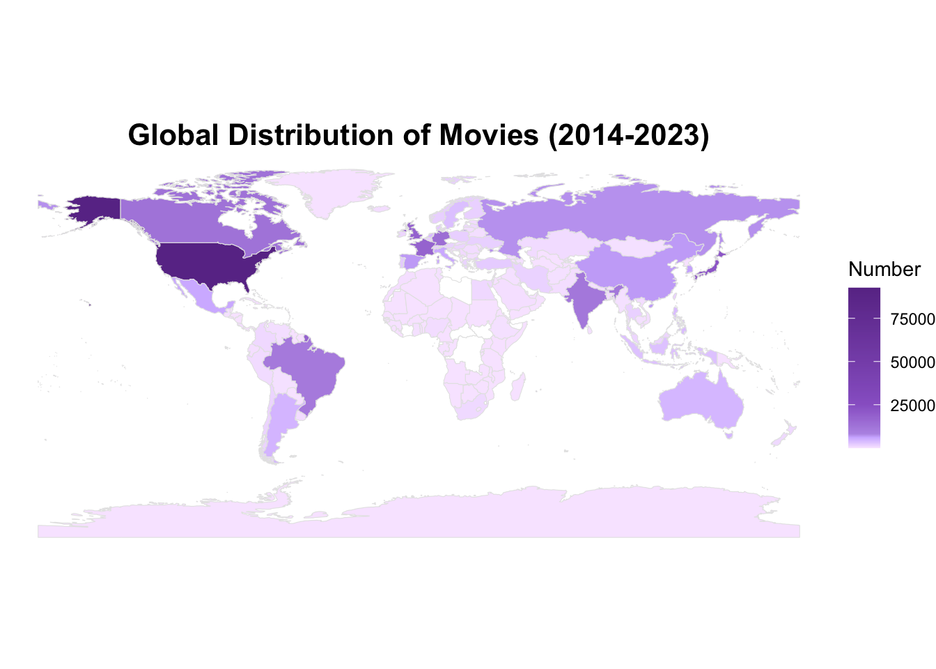
   country                  number
   <chr>                     <int>
 1 United States of America  92581
 2 Japan                     21813
 3 United Kingdom            17995
 4 France                    17648
 5 Germany                   14224
 6 Canada                    12759
 7 India                     11095
 8 Brazil                    10330
 9 Russia                     7140
10 Spain                      6608
# ℹ 222 more rows

world <- ne_countries(scale = "medium", returnclass = "sf")
world_data <- world |>
  left_join(df3, by = c("name" = "country"))

my_colors <- c(
  "#F8E8FF",  
  "#E4CFFF",  
  "#D1B7FF",  
  "#B998E6",  
  "#9966CC",  
  "#6A3795"   
)

value_points <- c(0, 3000, 6000, 8000, 25000, max(world_data$number, na.rm = TRUE))

ggplot(world_data) +
  geom_sf(aes(fill = number, geometry = geometry), color = "gray90", size = 0.1) +
  scale_fill_gradientn(
    colors = my_colors,
    values = scales::rescale(value_points),  
    na.value = "white"  
  ) +
  labs(
    title = "Global Distribution of Movies (2014-2023)",
    fill = "Number"
  ) +
  theme_void() +
  theme(
    plot.title = element_text(hjust = 0.5, size = 16, face = "bold")
  )

ggsave(
  filename = "data/Q3.png",
  plot = last_plot(),     
  width = 10, height = 6, dpi = 300     
)

Q4

In the past 15 years, what are the most profitable movie genres in China each year?

df4 <- df_clean |>
  select(year, genre, revenue, country) |>
  filter(country == "China") |>   
  filter(year>2013)|>
  group_by(year, genre) |>   
  summarise(total_revenue = sum(revenue)) |>  
  arrange(year, -total_revenue) |>     
  group_by(year) |>
  filter(!(year>2023))|>
  slice_max(order_by = total_revenue, n = 3) 

`summarise()` has grouped output by 'year'. You can override using the
`.groups` argument.

print(df4)

# A tibble: 30 × 3
# Groups:   year [10]
    year genre     total_revenue
   <dbl> <chr>             <dbl>
 1  2014 Comedy        305110001
 2  2014 Romance       270560150
 3  2014 Horror         65220000
 4  2015 Action        358300000
 5  2015 Romance       234050462
 6  2015 Adventure     223055045
 7  2016 Comedy        196653268
 8  2016 Action        103013412
 9  2016 Animation      87414558
10  2017 War           870322670
# ℹ 20 more rows

df4.3 <- df_clean |>
  select(year, genre, revenue, country) |>
  filter(country == "China") |>   
  filter(year>2008)|>
  group_by(year, genre) |>   
  summarise(total_revenue = sum(revenue)) |>  
  arrange(year, -total_revenue) |>     
  group_by(year) |>
  filter(!(year>2023))|>
  filter(genre %in% c(
    "Animation", "Drama", "Action", "War",  
    "Science Fiction", "Mystery", "Comedy"
  )) 

`summarise()` has grouped output by 'year'. You can override using the
`.groups` argument.

glimpse(df4.3)

Rows: 101
Columns: 3
Groups: year [15]
$ year          <dbl> 2009, 2009, 2009, 2009, 2009, 2009, 2010, 2010, 2010, 20…
$ genre         <chr> "Drama", "Action", "Animation", "Comedy", "Science Ficti…
$ total_revenue <dbl> 35450000, 16313580, 0, 0, 0, 0, 100297064, 5000000, 0, 0…

line_colors <- c(
  "#FFB6C1", "#B0E0E6",
  "#98FB98", "#D8BFD8", "#F0E68C",
  "#B998E6", "#87CEFA"
)

ggplot(df4.3, aes(x = year, y = total_revenue, color = genre, group = genre)) +
  geom_line(size = 0.8) +       
  geom_point(size = 2) +        
  scale_color_manual(values = line_colors) +  
  facet_wrap(~ genre, ncol = 1, scales = "fixed") +  # 按 genre 分面，统一 Y 轴
  scale_y_continuous(labels = scales::comma) +  # 格式化 Y 轴刻度为千分位
  scale_x_continuous(
    breaks = seq(2009, 2023, by = 2)  
  ) +
  labs(
    title = "Revenue Trends by Genre (2009-2023)",
    x = "Year",
    y = "Total Revenue"
  ) +
  theme_minimal() +
  theme(
    plot.title = element_text(hjust = 0.5, size = 10, face = "bold"),
    axis.text.x = element_text(size = 9),  
    axis.text.y = element_text(size = 8),  
    axis.title.x = element_text(hjust = 1, size = 12),  
    strip.text = element_text(size = 12, face = "bold"),  
    legend.position = "none"  
  )

Warning: Using `size` aesthetic for lines was deprecated in ggplot2 3.4.0.
ℹ Please use `linewidth` instead.

ggsave(
  filename = "data/Q4.png",
  plot = last_plot(),     
  width = 4, height = 7,dpi = 300     
)

Q5

Is there a relationship between a movie’s revenue and its rating?

df5 <- df_clean |>
  select(rate, revenue, title) |>  
  filter(!(rate == "NA"))|>
  filter(!(revenue<100001)) |>
  mutate(revenue = as.numeric(revenue))  
print(df5)

# A tibble: 1,266 × 3
    rate    revenue title                  
   <dbl>      <dbl> <chr>                  
 1   8   1518815515 The Avengers           
 2   8    783100000 Deadpool               
 3   8.4 2052415039 Avengers: Infinity War 
 4   8    772776600 Guardians of the Galaxy
 5   7.9  585174222 Iron Man               
 6   8.5  425368238 Django Unchained       
 7   8.4 2800000000 Avengers: Endgame      
 8   8.2  294800000 Shutter Island         
 9   8.2  392000000 The Wolf of Wall Street
10   7.3 1405403694 Avengers: Age of Ultron
# ℹ 1,256 more rows

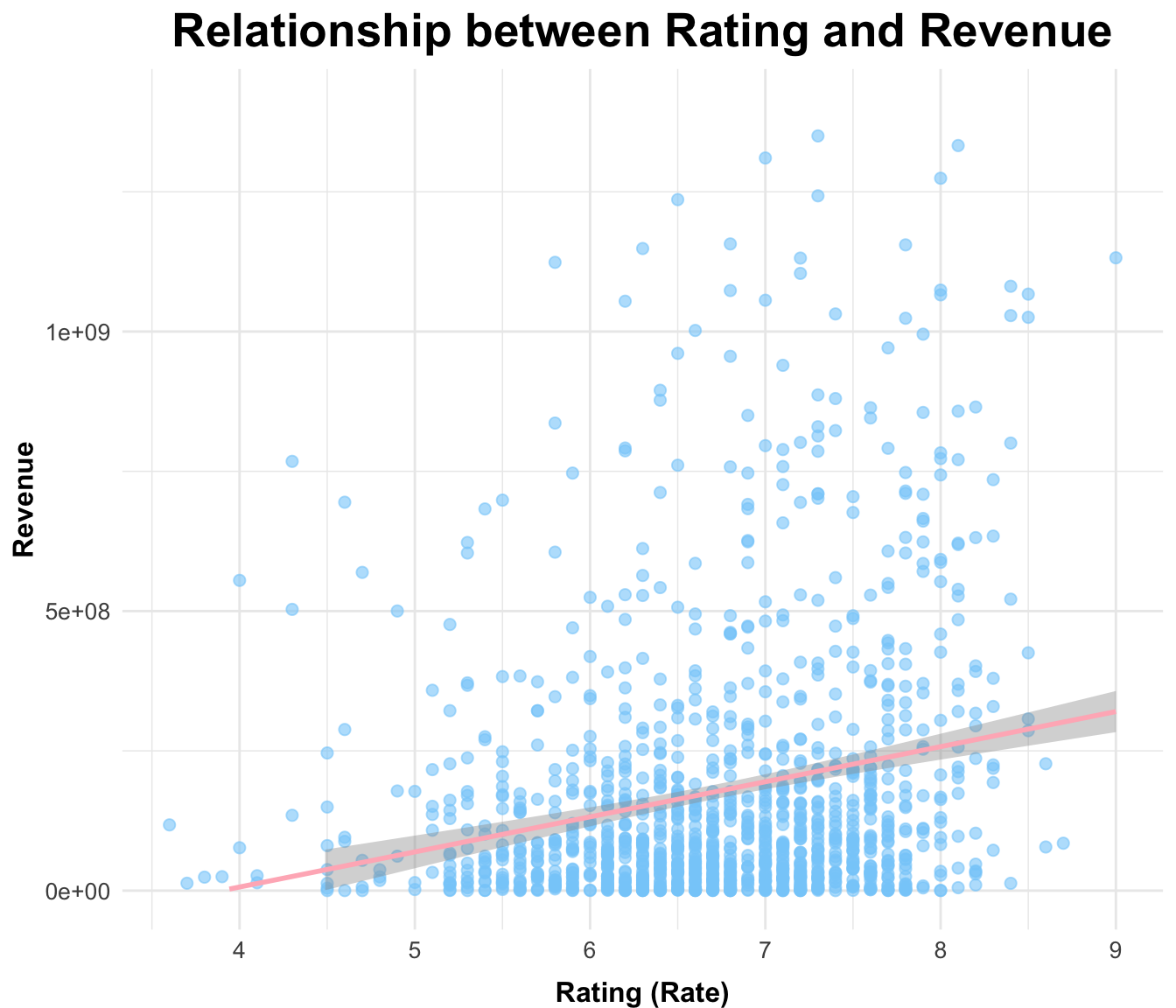
ggplot(df5, aes(x = rate, y = revenue)) +
  geom_point(color = "#87CEFA", alpha = 0.6, size = 2) +  
  geom_smooth(method = "lm", color =  "#FFB6C1") +  # 添加回归线
  labs(
    title = "Relationship between Rating and Revenue",
    x = "Rating (Rate)",
    y = "Revenue"
  ) +
  scale_y_continuous(limits= c(0, max(df5$revenue)*0.5)) +  # 设置Y轴上限为最大值的一半
  theme_minimal() +
  theme(
    # 图表标题：大字体，居中，上对齐
    plot.title = element_text(hjust = 0.5, vjust = 1, size = 20, face = "bold"),
    # Y轴标题：大字体，上对齐
    axis.title.y = element_text(size = 12, hjust = 0.5, vjust = 1, angle = 90, face = "bold"),
    axis.text.y = element_text(size = 10),
    # X轴标题：大字体，下对齐
    axis.title.x = element_text(size = 12, hjust = 0.5, vjust = -1, face = "bold"),
    axis.text.x = element_text(size = 10)
  )

`geom_smooth()` using formula = 'y ~ x'

Warning: Removed 11 rows containing non-finite outside the scale range
(`stat_smooth()`).

Warning: Removed 11 rows containing missing values or values outside the scale range
(`geom_point()`).

Warning: Removed 5 rows containing missing values or values outside the scale range
(`geom_smooth()`).

ggsave(
  filename = "data/Q5.png",
  plot = last_plot(),     
  dpi = 300     
)

Saving 7 x 5 in image
`geom_smooth()` using formula = 'y ~ x'

Warning: Removed 11 rows containing non-finite outside the scale range
(`stat_smooth()`).

Warning: Removed 11 rows containing missing values or values outside the scale range
(`geom_point()`).

Warning: Removed 5 rows containing missing values or values outside the scale range
(`geom_smooth()`).